Let’s explain by way of example. Suppose your uncle entrusted you with his Mercedes for the summer. He heads for the Bahamas and says, “I’ll see you in the fall.” At that time, Mercedes are in short supply, and the going rate is about $30,000 to own this fine automobile.
Unknown to your uncle, you sell his car and put the money in your bank account, earning interest. Now, come August, the Mercedes supply problem has been solved, so there are more of them on the market. You go out and buy the Mercedes back for $25,000. Your uncle returns, gets his car, and you pocket $5,000.
That’s how short selling works—you borrow stock from your broker (owned by somebody else) and sell it to the market. You owe the broker the stock. Later, you hope to buy it back (from the market) and replenish the stock you borrowed. If it is priced lower at that point, you pocket the difference.
However, what happens if the item is pricier in the future? Let’s say that there is a sudden run on Mercedes in early August, and it costs you $35,000 to buy one. You must come up with this money, so you will suffer a $5,000 loss. In the same way, if you short stock and it goes up, you will lose the difference at the point you “cover” your short sale.
Imagine we’re flipping a coin. Heads I win one and – Tails you win. Simple. Heads and tails will each come up half the time, and we’ll both neither win or loss.
However, unknown to me, you have a loaded coin. For ever 100 throws, heads comes up 49 and tails comes 51 times.
You now have a license to print money. Let’s call it the “Tails Trading System”.
All you have to do is sit back and bet on tails forever. Eventually, You’d win all my money(and anyone else’s who took you on).
All any trading system gives you is an “EDGE”. A favorable bias. Something that is more likely to happen than out.
You are relying on a positive bias, essentially, the trading system “when ‘X’ happens…’Y’ usually follows”.
sometimes it doesn’t work. Most of the time is does.
And all your trading does in help you identify high probability trades, enter then correctly, and protect yourself while allowing your profits to grow”.
Now some trading systems ae better than others. But don’t get caught up on the search for the perfect system…..
Find a trading system that you like. one you feel comfortable with. one you understand. Then stick with it. Be Consistent.
A cool, disciplined, trader will take an average system and make money with it, A nervous, arbitrary trader will take a brilliant system and wreck it.
All traders have “good” days and “bad” days. Some days you’ll make small profits, other day you’ll make small losses. And once or twice a month, on average, you’ll make big profit. That’s how you make money as a trader, It’s not 9 till 4.
Problem is, you never know when the big traders are due to arrive. Like out “Tails Trading System” Above, the one time you don’t take the trade is exactly the time the market takes off and never looks back.
You MUST see the big picture. Realize that the current trade is only one of many. On that basis, the current trade hardly matters. It’s like a piece of plankton in a very large OCEAN.
Trading is all about managing risk and then surrendering yourself to the oldest law in the universe.
So today, I’m here to go through everything that’s on my desk!
My desk is where I do most of my thinking and creating. It’s a representation of the writer, blogger, and reader in me, and just like the constant changes made in my inspiration and creativity process, my desk is a space that also needs to be changed and altered constantly. The things that are on my desk each have their own personal meaning and reason as to why they are put on my desk in the first place. Each item also inspire me in different ways
Any who, whether you’re here to look for some desk inspiration or find out more about what’s on my desk, lets jump out of this post!
This is my very first self-purchased plant baby! I put them on my desk because because I wanted something that could grow along with me A little cheesy, but it motivates me to work and strive for the best! I’m also sentimental over the fact and Now I’m just way too attached!
I also have these headphones, but these headphones are a huge plus because they are noise-cancelling and, of course, wireless. I need them almost every time I blog or study!
I also have my trusty journal with me on my desk! I use my journal almost daily for both blogging and personal reasons. I love anything to do with journaling, so having a journal near me is very important!
I also have of books with different genres like Finance, Biographies, Romantic and Mysterious and Horror and lot.
This are the major thing are on my desk which inspire to me a lot.
My planner is one of those simple to read good books which are based on Finance, Psychology, Behavioral Science & done all the work Which I have. Make Sketches and Create an ideas for blog posts.
Microsoft Excel is the most important tool of Investment Bankers and Financial Analysts. They spent more than 70% of the time preparing Excel Models, formulating Assumptions, Valuations, Calculations, Graphs, etc. It is safe to assume that Investment bankers are masters in excel shortcuts and formulas. Though there are more than 50+ Financial Functions in Excel, here is the list of Top 15 financial functions in excel that are most frequently used in practical situations.
Without much ado, let’s have a look at all the financial functions one by one –
#1 – Future Value (FV)
#2 – FVSCHEDULE
#3 – Present Value (PV)
#4 – Net Present Value (NPV)
#5 – XNPV
#6 – PMT
#7 – PPMT
#8 – Internal Rate of Return (IRR)
#9 – Modified Internal Rate of Return (MIRR)
#10 – XIRR
#11 – NPER
#12 – RATE
#13 – EFFECT
#14 – NOMINAL
#15 – SLN
#1 – Future Value (FV): Financial Function in Excel
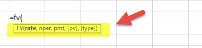
If you want to find out the future value of a particular investment which has a constant interest rate and periodic payment, use the following formula –
FV (Rate, Nper, [Pmt], PV, [Type])
Rate = It is the interest rate/period
Nper = Number of periods
[Pmt] = Payment/period
PV = Present Value
[Type] = When the payment is made (if nothing is mentioned, it’s assumed that the payment has been made at the end of the period)
FV Example
A has invested the US $100 in 2017. The payment has been made yearly. The interest rate is 10% p.a. What would be the FV in 2020?
Solution: In excel, we will put the equation as follows –
= FV (10%, 3, 1, – 100)
= US $129.79
#2 – FVSCHEDULE: Financial Function in Excel
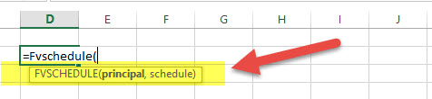
This financial function is important when you need to calculate the future value with the variable interest rate. Have a look at the function below –
FVSCHEDULE = (Principal, Schedule)
Principal = Principal is the present value of a particular investment
Schedule = A series of interest rate put together (in case of excel, we will use different boxes and select the range)
FVSCHEDULE Example:
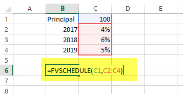
M has invested the US $100 at the end of 2017. It is expected that the interest rate will change every year. In 2018, 2019 & 2020, the interest rates would be 4%, 6% & 5% respectively. What would be the FV in 2020?
Solution: In excel, we will do the following –
= FVSCHEDULE (C1, C2: C4)
= US $115.752
#3 – Present Value (PV): Financial Function in Excel
If you know how to calculate FV, it’s easier for you to find out PV. Here’s how –
PV = (Rate, Nper, [Pmt], FV, [Type])
Rate = It is the interest rate/period
Nper = Number of periods
[Pmt] = Payment/period
FV = Future Value
[Type] = When the payment is made (if nothing is mentioned, it’s assumed that the payment has been made at the end of the period)
PV Example:
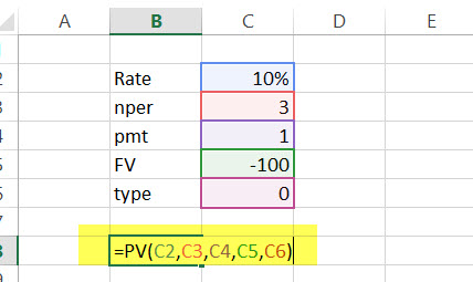
The future value of an investment in the US $100 in 2020. The payment has been made yearly. The interest rate is 10% p.a. What would be the PV as of now?
Solution: In excel, we will put the equation as follows –
= PV (10%, 3, 1, – 100)
= US $72.64
#4 – Net Present Value (NPV): Financial Function in Excel
Net Present Value is the sum total of positive and negative cash flows over the years. Here’s how we will represent it in excel –
NPV = (Rate, Value 1, [Value 2], [Value 3]…)
Rate = Discount rate for a period
Value 1, [Value 2], [Value 3]… = Positive or negative cash flows
Here, negative values would be considered as payments and positive values would be treated as inflows.
NPV Example
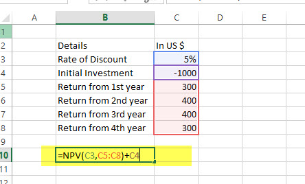
Here is a series of data from which we need to find NPV –
Details
In US $
Rate of Discount
5%
Initial Investment
-1000
Return from 1st year
300
Return from 2nd year
400
Return from 3rd year
400
Return from 4th year
300
Find out the NPV.
Solution: In Excel, we will do the following –
=NPV (5%, B4:B7) + B3
= US $240.87
Also, have a look at this article – NPV vs IRR
#5 – XNPV: Financial Function in Excel
This financial function is similar as the NPV with a twist. Here the payment and income are not periodic. Rather specific dates are mentioned for each payment and income. Here’s how we will calculate it –
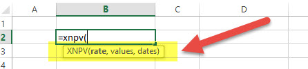
XNPV = (Rate, Values, Dates)
Rate = Discount rate for a period
Values = Positive or negative cash flows (an array of values)
Dates = Specific dates (an array of dates)
XNPV Example
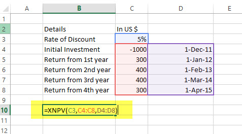
Here is a series of data from which we need to find NPV –
Details
In US $
Dates
Rate of Discount
5%
Initial Investment
-1000
1st December 2011
Return from 1st year
300
1st January 2012
Return from 2nd year
400
1st February 2013
Return from 3rd year
400
1st March 2014
Return from 4th year
300
1st April 2015
Solution: In excel, we will do as follows –
=XNPV (5%, B2:B6, C2:C6)
= US$289.90
#6 – PMT: Financial Function in Excel
In excel, PMT denotes the periodical payment required to pay off for a particular period of time with a constant interest rate. Let’s have a look at how to calculate it in excel –
PMT = (Rate, Nper, PV, [FV], [Type])
Rate = It is the interest rate/period
Nper = Number of periods
PV = Present Value
[FV] = An optional argument which is about the future value of a loan (if nothing is mentioned, FV is considered as “0”)
[Type] = When the payment is made (if nothing is mentioned, it’s assumed that the payment has been made at the end of the period)
PMT Example
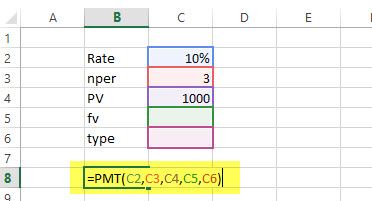
US $1000 needs to be paid in full in 3 years. The interest rate is 10% p.a. and the payment needs to be done yearly. Find out the PMT.
Solution: In excel, we will calculate it in the following manner –
= PMT (10%, 3, 1000)
= – 402.11
#7 – PPMT: Financial Function in Excel
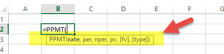
It is another version of PMT. The only difference is this – PPMT calculates payment on principal with a constant interest rate and constant periodic payments. Here’s how to calculate PPMT –
PPMT = (Rate, Per, Nper, PV, [FV], [Type])
Rate = It is the interest rate/period
Per = The period for which the principal is to be calculated
Nper = Number of periods
PV = Present Value
[FV] = An optional argument which is about the future value of a loan (if nothing is mentioned, FV is considered as “0”)
[Type] = When the payment is made (if nothing is mentioned, it’s assumed that the payment has been made at the end of the period)
PPMT Example
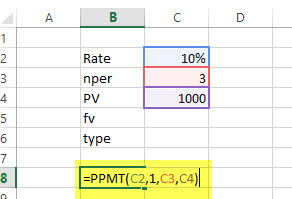
US $1000 needs to be paid in full in 3 years. The interest rate is 10% p.a. and the payment needs to be done yearly. Find out the PPMT in the first year and second year.
Solution: In excel, we will calculate it in the following manner –
1st year,
=PPMT (10%, 1, 3, 1000)
= US $-302.11
2nd year,
=PPMT (10%, 2, 3, 1000)
= US $-332.33
#8 – Internal Rate of Return (IRR): Financial Function in Excel
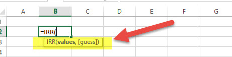
To understand whether any new project or investment is profitable or not, the firm uses IRR. If IRR is more than the hurdle rate (acceptable rate/ average cost of capital), then it’s profitable for the firm and vice-versa. Let’s have a look, how we find out IRR in excel –
IRR = (Values, [Guess])
Values = Positive or negative cash flows (an array of values)
[Guess] = An assumption of what you think IRR should be
IRR Example
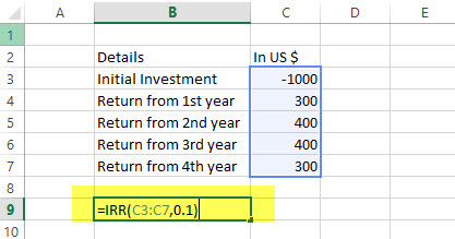
Here is a series of data from which we need to find IRR –
Details
In US $
Initial Investment
-1000
Return from 1st year
300
Return from 2nd year
400
Return from 3rd year
400
Return from 4th year
300
Find out IRR.
Solution: Here’s how we will calculate IRR in excel –
= IRR (A2:A6, 0.1)
= 15%
#9 – Modified Internal Rate of Return (MIRR): Financial Function in Excel
Modified Internal Rate of Return is one step ahead of the Internal Rate of Return. MIRR signifies that the investment is profitable and is used in business. MIRR is calculated by assuming NPV as zero. Here’s how to calculate MIRR in excel –
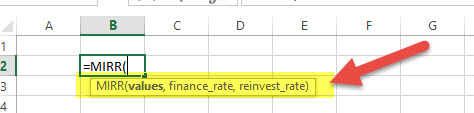
MIRR = (Values, Finance rate, Reinvestment rate)
Values = Positive or negative cash flows (an array of values)
Finance rate = Interest rate paid for the money used in cash flows
Reinvestment rate = Interest rate paid for reinvestment of cash flows
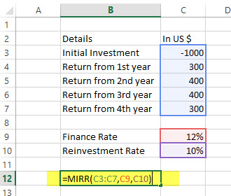
MIRR Example
Here is a series of data from which we need to find MIRR –
Here we need to find out IRR which has specific dates of cash flow. That’s the only difference between IRR and XIRR. Have a look at how to calculate XIRR in excel financial function –
XIRR = (Values, Dates, [Guess])
Values = Positive or negative cash flows (an array of values)
Dates = Specific dates (an array of dates)
[Guess] = An assumption of what you think IRR should be
XIRR Example
Here is a series of data from which we need to find XIRR –
Details
In US $
Dates
Initial Investment
-1000
1st December 2011
Return from 1st year
300
1st January 2012
Return from 2nd year
400
1st February 2013
Return from 3rd year
400
1st March 2014
Return from 4th year
300
1st April 2015
Solution: Let’s have a look at the solution –
= XIRR (B2:B6, C2:C6, 0.1)
= 24%
#11 – NPER: Financial Function in Excel
It is simply the number of periods one requires to pay off the loan. Let’s see how we can calculate NPER in excel –
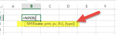
NPER = (Rate, PMT, PV, [FV], [Type])
Rate = It is the interest rate/period
PMT = Amount paid per period
PV = Present Value
[FV] = An optional argument which is about the future value of a loan (if nothing is mentioned, FV is considered as “0”)
[Type] = When the payment is made (if nothing is mentioned, it’s assumed that the payment has been made at the end of the period)
NPER Example
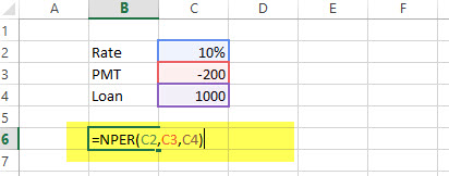
US $200 is paid per year for a loan of US $1000. The interest rate is 10% p.a. and the payment needs to be done yearly. Find out the NPER.
Solution: We need to calculate NPER in the following manner –
= NPER (10%, -200, 1000)
= 7.27 years
#12 – RATE: Financial Function in Excel
Through the RATE function in excel, we can calculate the interest rate needed to pay off the loan in full for a given period of time. Let’s have a look at how to calculate RATE financial function in excel –
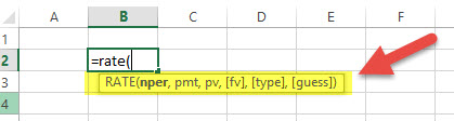
RATE = (NPER, PMT, PV, [FV], [Type], [Guess])
Nper = Number of periods
PMT = Amount paid per period
PV = Present Value
[FV] = An optional argument which is about the future value of a loan (if nothing is mentioned, FV is considered as “0”)
[Type] = When the payment is made (if nothing is mentioned, it’s assumed that the payment has been made at the end of the period)
[Guess] = An assumption of what you think RATE should be
RATE Example
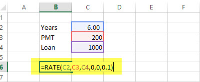
US $200 is paid per year for a loan of US $1000 for 6 years and the payment needs to be done yearly. Find out the RATE.
Solution:
= RATE (6, -200, 1000, 0.1)
= 5%
#13 – EFFECT: Financial Function in Excel
Through the EFFECT function, we can understand the effective annual interest rate. When we have the nominal interest rate and the number of compounding per year, it becomes easy to find out the effective rate. Let’s have a look at how to calculate EFFECT financial function in excel –
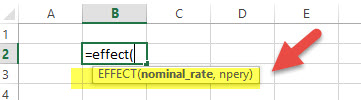
EFFECT = (Nominal_Rate, NPERY)
Nominal_Rate = Nominal Interest Rate
NPERY = Number of compounding per year
EFFECT Example
Payment needs to be paid with a nominal interest rate of 12% when the number of compounding per year is 12.
Solution:
= EFFECT (12%, 12)
= 12.68%
#14 – NOMINAL: Financial Function in Excel
When we have an effective annual rate and the number of compounding periods per year, we can calculate the NOMINAL rate for the year. Let’s have a look at how to do it in excel –
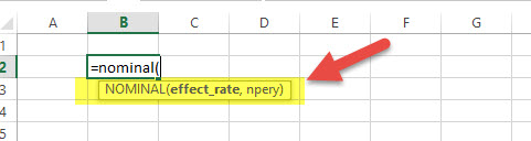
NOMINAL = (Effect_Rate, NPERY)
Effect_Rate = Effective annual interest rate
NPERY = Number of compounding per year
NOMINAL Example
Payment needs to be paid with an effective interest rate or annual equivalent rate of 12% when the number of compounding per year is 12.
Solution:
= NOMINAL (12%, 12)
= 11.39%
#15 – SLN: Financial Function in Excel
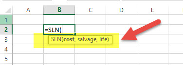
Through the SLN function, we can calculate depreciation via a straight-line method. In excel, we will look at SLN financial function as follows –
SLN = (Cost, Salvage, Life)
Cost = Cost of asset when bought (initial amount)
Salvage = Value of asset after depreciation
Life = Number of periods over which the asset is being depreciated
SLN Example
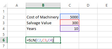
The initial cost of machinery is the US $5000. It has been depreciated in the Straight Line Method. The machinery was used for 10 years and now the salvage value of machinery is the US $300. Find depreciation charged per year.